Overview

Simulations are organized into sets. Sets have names like emulator_1100box_planck, and simulations have numbers appended to them, like emulator_1100box_planck_00. A dash after the number (like emulator_1100box_planck_00-1) means this is a different phase of the same cosmology; that is, an independent realization of the power spectrum.

Simulation Sets

Simulation Set Name	# of sims	Box Size [\(\mathrm{Mpc}/h\)]	\(N_\mathrm{part}\)	Particle Mass [\(M_\odot/h\)]	Cosmologies	Initial Phases	Output Redshifts	Notes	Softening
AbacusCosmos_1100box (Browse)	41	1100	\(1440^3\)	\(\sim 4\times 10^{10}\)	Latin Hypercube centered on Planck 2015	Matched	1.5, 1.0, 0.7, 0.5, 0.3		Spline, \(63\;\mathrm{kpc}/h\)
AbacusCosmos_720box (Browse)	41	720	\(1440^3\)	\(\sim 1\times 10^{10}\)	Latin Hypercube centered on Planck 2015	Matched	1.5, 1.0, 0.7, 0.5, 0.3, 0.1	Not zoom-in boxes of the above	Spline, \(41\;\mathrm{kpc}/h\)
AbacusCosmos_1100box_planck (Browse)	20	1100	\(1440^3\)	\(\sim 4\times 10^{10}\)	Fiducial	Independent	1.5, 1.0, 0.7, 0.5, 0.3		Spline, \(63\;\mathrm{kpc}/h\)
AbacusCosmos_720box_planck (Browse)	20	720	\(1440^3\)	\(\sim 1\times 10^{10}\)	Fiducial	Independent	1.5, 1.0, 0.7, 0.5, 0.3, 0.1	Not zoom-in boxes of the above	Spline, \(41\;\mathrm{kpc}/h\)
emulator_1100box_planck_00-{0..15} (Browse)	16	1100	\(1440^3\)	\(\sim 4\times 10^{10}\)	Fiducial	Independent	0.7, 0.57, 0.5, 0.3	Volume-building boxes	Plummer, \(63\;\mathrm{kpc}/h\)
emulator_1100box_planck_{00..04} (Browse)	5	1100	\(1440^3\)	\(\sim 4\times 10^{10}\)	Fiducial + perturbations	Matched	0.7, 0.57, 0.5, 0.3	Derivative-measuring boxes	Plummer, \(63\;\mathrm{kpc}/h\)
emulator_720box_planck_00-{0..15} (Browse)	16	720	\(1440^3\)	\(\sim 1\times 10^{10}\)	Fiducial	Independent	0.7, 0.57, 0.5, 0.3, 0.1	Volume-building boxes	Plummer, \(41\;\mathrm{kpc}/h\)
emulator_720box_planck_{00..04} (Browse)	5	720	\(1440^3\)	\(\sim 1\times 10^{10}\)	Fiducial + perturbations	Matched	0.7, 0.57, 0.5, 0.3, 0.1	Derivative-measuring boxes	Plummer, \(41\;\mathrm{kpc}/h\)

Design

The 40 AbacusCosmos simulations are designed to allow estimation of derivatives of cosmological measurables with respect to cosmology. They can either be used as an ensemble to construct an emulator/interpolator, or each individual box can be differenced with the central AbacusCosmos_planck box to provide an estimate of the derivative for that particular change in cosmology.

The boxes do not provide much volume of any individual cosmology (\(1.7\;(\mathrm{Gpc}/h)^3\) if both resolutions are combined), but the 20 AbacusCosmos_planck boxes and 16 emulator_planck boxes with independent phases provide additional volume and a path toward suppressing cosmic variance and estimating covariance. The 5 emulator_planck single-parameter excursion boxes provide a more direct route to measuring derivatives but only for two parameters. The AbacusCosmos boxes are more modern than the emulator_planck boxes in that they all use spline softening, which alleviates many “over-softening” issues with Plummer softening (see Softening).

The motivation for two mass resolutions was first to provide a convergence test for large-scale structure properties, at least in the intermediate regime well-sampled by both resolutions. Second, the larger boxes provide the volume that is needed for BAO-type studies, while the smaller boxes provide the halo resolution that is needed by weak lensing studies.

In general, the lowest redshift slice (usually \(z=0.1\)) is only available for the smaller (720 Mpc/h) boxes, since the amount of observable cosmological volume is relatively small by that redshift. Thus, the smaller boxes are usually sufficient and also offer better resolution.

Cosmologies

Fiducial Cosmology

The fiducial cosmology is taken from the Planck 2015 cosmological parameters paper. This is the cosmology of the emulator_planck_00 sims and the AbacusCosmos_planck sims. The AbacusCosmos sims use 40 cosmologies scattered around this cosmology.

The cosmological parameters are listed here for convenience, but in analysis applications the cosmological parameters should always be read from abacus.par or camb_params.ini.

Parameter	Value
ombh^2	0.02222
omcdmh^2	0.1199
omh^2	0.14212
w0	-1.0
ns	0.9652
sigma_8	0.830
H0	67.26
N_eff	3.04
massless_neutrinos	3.04
omnuh2	0.0

Fiducial + perturbations

The emulator_planck_{00..04} boxes provide a central cosmology and four perturbations: \(\sigma_8 \pm 5\%\) and \(H_0 \pm 5\%\). Thus, these 5 boxes form a “plus sign” of cosmologies.

The perturbations are listed here. Note that since the cosmologies are chosen in the space of physical densities, changes to \(H_0\) result in changes to \(\Omega_m, \Omega_\Lambda\).

Sim	\(H_0\)	\(\Omega_\mathrm{DE}\)	\(\Omega_M\)	\(\sigma_8\)
00 (fiducial)	67.3	0.686	0.314	0.83
01	67.3	0.686	0.314	0.78
02	67.3	0.686	0.314	0.88
03	64.3	0.656	0.344	0.83
04	70.3	0.712	0.288	0.83

AbacusCosmos Cosmologies

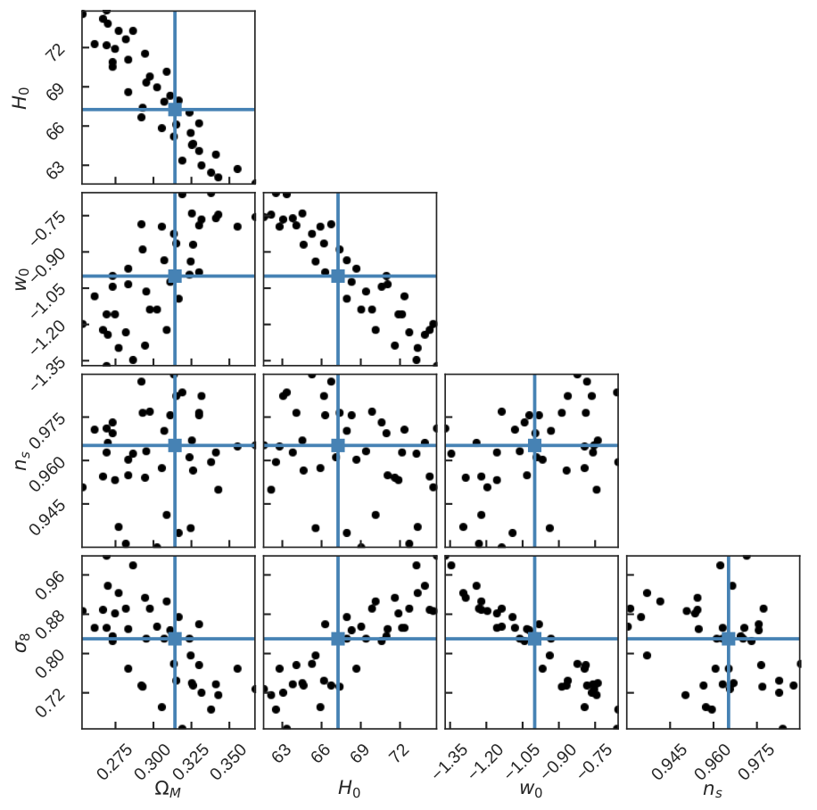
The AbacusCosmos_1100box and AbacusCosmos_720box sims use a set of 40 cosmologies chosen with a Latin hypercube algorithm centered on the Planck 2015 cosmology. We vary \(H_0\), \(w_0\), \(\Omega_\mathrm{CDM}h^2\), \(\Omega_bh^2\), \(\sigma_8\), and \(n_s\). The cosmology of a given simulation can be read from the info/abacus.par file. The full list of cosmologies is available here.

Below we show a corner plot representation of this 6-dimensional parameter space, where we have combined \(\Omega_\mathrm{CDM}\) and \(\Omega_b\) into \(\Omega_M\). The blue square marks the AbacusCosmos_planck simulation, which is a realization of the fiducial cosmology that is phase-matched to the rest of the AbacusCosmos sims.

Softening

The Abacus Cosmos suite employs two force softening techniques: Plummer and spline. The AbacusCosmos sims use spline, while the emulator_planck sims use Plummer. We generally consider spline to be more physically accurate than Plummer on small scales because the long tail of the Plummer force law suppresses power relative to spline, even for the same Plummer-equivalent softening length. However, our fast spline implementation was only developed partway through the simulation effort and was thus only applied to the remaining sims. In general, our softening lengths were chosen to support halos, not subhalos.

Softening lengths (spline or Plummer) are always quoted in Plummer-equivalent units, meaning we match the minimum dynamical time for particle orbits.

Plummer softening

In Plummer softening, the \(\mathbf{F}(\mathbf{r}) = \mathbf{r}/r^3\) force law is modified as

\(\mathbf{F}(\mathbf{r}) = \frac{\mathbf{r}}{(r^2 + \epsilon_p^2)^{3/2}}\),

where \(\epsilon_p\) is the softening length. Note that this form is not compact, meaning it never explicitly switches to the \(r^{-2}\) form at any radius.

Spline softening

In spline softening, the force law is a piecewise function that explicitly switches to \(r^{-2}\) at a certain radius. Traditional spline implementations have three or more piecewise segments, but this can be slow in practice. We only include two piecewise segments and require continuity and smoothness at the transition up to the second derivative. Because we split only once, we call our form “single spline”. The law is derived from a Taylor expansion in \(r\) of Plummer softening and is as follows:

\[\mathbf{F}(\mathbf{r}) = \begin{cases} \left(10 - 15(r/\epsilon_s) + 6(r/\epsilon_s)^2\right)\mathbf{r}/\epsilon_s^3, & r < \epsilon_s; \\ \mathbf{r}/r^3, & r >= \epsilon_s. \end{cases}\]

Initial Conditions

The initial conditions were generated by the public zeldovich-PLT code of Garrison+2016. We do not provide initial conditions files with the catalogs, but we do provide the input parameter file (info/abacus.par) for the IC code and the input power spectrum from CAMB. The initial conditions can thus be generated by re-running the IC code with those inputs; see below.

The simulations use second-order Lagrangian perturbation theory (2LPT) initial conditions, but zeldovich-PLT only outputs first order displacements. The 2LPT corrections are generated by Abacus on-the-fly using the configuration-space method of Garrison+2016.

Two non-standard first-order corrections are implemented by zeldovich-PLT. The first is that the displacements use the particle lattice eigenmodes rather than the curl-free continuum eigenmodes. This eliminates transients that arise due to the discretization of the continuum dynamical system (the Vlasov-Boltzmann distribution function) into particles on small scales near \(k_\mathrm{Nyquist}\). The second correction is “rescaling”, in which initial mode amplitudes are adjusted to counteract the violation of linear theory that inevitably happens on small scales in particle systems. This violation usually takes the form of growth suppression; thus the initial adjustments are mostly amplitude increases. We choose \(z_\mathrm{target} = 5\) as the redshift at which the rescaled solution will match linear theory; this choice is tested in Garrison+2016.

Some simulations are referred to as “phase-matched” in the initial conditions. This refers to initial conditions with the same random number generator seed, called ZD_Seed in the abacus.par file. Matching this value (and ZD_NumBlock) between two simulations guarantees that the amplitudes and phases of the initial modes are identical between the simulations (up to differences in the input power spectrum and cosmology).

Re-generating ICs

To re-generate the initial conditions for a given sim, make a copy of the abacus.par file from the simulation and pass it as the parameter file to the zeldovich-PLT code. Most of the parameters will not need modification, but any parameters related to file paths will have to be modified to suit your system. Specifically, the following will likely need to be updated:

• InitialConditionsDirectory: The output directory for the IC files.
• ZD_PLT_filename: The PLT eigenmodes file. This is included with the zeldovich-PLT code (probably eigmodes128).
• ZD_Pk_filename: The input power spectrum file (i.e. the CAMB output file). This is included with each sim as info/camb_matterpower.dat.

Furthermore, zeldovich-PLT underwent an upgrade in November 2019, rendering it necessary to specify ZD_Version = 1 to generate legacy AbacusCosmos ICs. The code will not run if ZD_Version is absent.

Note about *-0 simulations

Due to an oversight in an earlier version of zeldovich-PLT, ZD_Seed = 0 used a time-based seed whose value was not logged. Thus, it is impossible to reconstruct intial conditions for those sims. This should only affect the emulator*00-0 boxes; none of the more recent simulations use ZD_Seed = 0.

Power Spectra

We use CAMB to generate a linear \(z=0\) power spectrum for each cosmology in our grid. We then scale the power spectrum back to \(z_\mathrm{init}=49\) by scaling \(\sigma_8\) by the ratio of the growth factors \(D(z=49)/D(z=0)\). This \(\sigma_8\) is passed to zeldovich-PLT, which handles the re-normalization of the power spectrum. The computation of the growth factors is done by Abacus’s cosmology module, so it is consistent by construction with the simulation’s cosmological evolution. We only use massless neutrinos and include no cosmological neutrino density. The exact CAMB inputs and outputs are available with each simulation (info/camb_params.ini and related info/camb_* files; see Info Directory).